After an awesome first day, the second day continued to carry forward the momentum. We had Vinay Malvimat’s second talk on entanglement — with a guest appearance by Ronak M Soni (TIFR) — and Sudip Ghosh (ICTS) giving the second talk on scattering amplitudes and the CHY formula; finally, in the evening, Pratik Roy (IoP) began his three-lecture series on anomalies.
Vinay began by motivating and introducing the Ryu-Takayanagi formula for calculating the entanglement of a holographic CFT using the AdS/CFT correspondence. The formula is that the entanglement of a region in the boundary with its complement is proportional to the area of the minimal-area surface in the bulk whose boundary is on the boundary of the region of interest,

An important stipulation here is that the minimal area surface be “homologous” to the boundary region whose entanglement we’re calculating, which basically means that there should be no black hole between the minimal area surface and the region (making this one of the rare occasions in physics in which a black hole is actually a hole). While this may sound arbitrary, there’s a deep reason for this. In a pure state, all the entropy normally called entanglement comes from the correlations between the region and its complement, because of which both the region and the complement have the same entropy. In a thermal state (which in the bulk looks like a black hole), however, the quantity called entanglement entropy mixes up thermal entropy and quantum correlations; because of this, the region and the complement usually have different entropies. If we naively use the minimal area surface in any background, the region and the complement always have the same entropy. In other words, this stipulation ensures that that mixed states don’t look pure.
(No one thought to ask the question of what happens at small non-zero temperatures when there’s no black hole in the bulk.)
He motivated it using the twist operator formalism in 2d CFT he showed us yesterday. First he reminded us that he’d shown us yesterday that the entanglement is the two-point function of two twist operators (operators at the ends of a region of interest that impose the boundary conditions required to calculate the replica trick path integral). Then, he explained that in 


Having given the audience of physicists a physicists’ proof (also known as a plausibility argument by our more enlightened colleagues), he showed us that it exactly reproduces the vacuum and thermal state entanglement entropies he’d derived in 2d CFT yesterday by explicitly solving for the minimal area surface. Then, he also calculated vacuum and thermal state entropy for a strip-shaped region of a CFT in any dimension. Finally, we had a coffee break.
Just before the coffee break, there had been questions about whether the Ryu-Takayanagi formula had been proved; it had been proved by Lewkowycz and Maldacena in 2013. Since Vinay was not very familiar with the paper and he’d covered the ground he’d wanted to cover for the day, Ronak M Soni (TIFR) decided to give a rough (to put it mildly) overview of the proof.
He began by explaining how the replica trick can be thought of as a path integral on a manifold that looks conical when one is near the entangling surface; the singularity analgous to the tip of a cone is located at the entangling surface and the circle direction of the cone is going around it in the two directions transverse to the entangling surface. In an n-sheeted cover of the original manifold, going around the entangling surface requires one to traverse an angle 
Then, he showed us how the Einstein-Hilbert action behaved on a manifold with a conical singularity; it splits into an integral of the Ricci scalar in the smooth region (the entire integral just scales as n times the integral on the original un-replicated manifold, because locally the two spaces are the same, but there’s n times more of the replicated space) and a piece localised on the singularity,
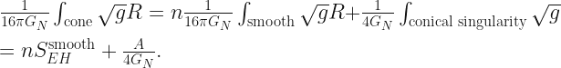
For a moment pretending that this action is the replica free energy 
In lieu of answering that question, Ronak took the CFT on the replicated manifold and asked what its bulk dual was. The bulk dual is an AdS geometry that looks like the replicated manifold on the boundary and solves the bulk Einstein equations. However, because of the particular geometry of AdS at the boundary, this solution is smooth and doesn’t have the conical singularity. Thus, the math he’d done earlier was still not applicable.
The crucial observation was that even though this manifold didn’t have a conical singularity, it was still like a smoothed out cone; the replicated manifold had a 
The second session was a talk by Sudip Ghosh (ICTS) on motivating the CHY formalism by explaining its connection to string theory. He approached it in two directions, by showing that a particularly simple amplitude in Yang-Mills theory had a stringy interpretation, and by showing that you could make a simple modification to a string theory amplitude and obtain a Yang-Mills amplitude.
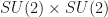
First, he introduced the spinor helicity formalism that makes amplitude calculations for massless particles particularly easy. Writing the Lorentz group 


Then, he showed us the form of the maximally helicity-violating (MHV) amplitude, an n-point amplitude in which all but two particles have positive helicity,

Then, by introducing a Lagrange multiplier for the total momentum-conservation delta function (which has the interpretation of a point in spacetime!) and Fourier transforming 


To interpret this, he introduced the space of all null rays in spacetime, also called twistor space; it’s isomorphic to 


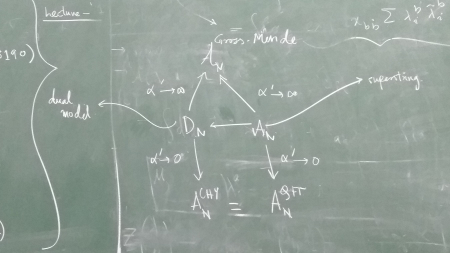
Having shown this relation to string theory, he went to the calculation of a tree-level amplitude in open string theory and reviewed Gross and Mende’s work on how the high-energy limit makes the moduli space integration localise onto solutions of the scattering equations introduced by Arnab in his talk. For standard reasons, in the low-energy limit this amplitude just become the Yang-Mills amplitude.
Then he explained Bjerrum-Bohr’s modification of this amplitude by adding a delta function factor in the integrand localising the integral onto the solutions of the scattering equations. The marvellous thing about this modification is that in the high energy limit it exactly reproduces the Gross-Mende answer, and in the low-energy limit it exactly reproduces the CHY answer for the Yang-Mills amplitude!
While, because of the saddle-point analysis of Gross and Mende, the coincidence in the high energy limit is easy to see, the coincidence in the low energy limit is not understood very well. This extremely non-trivial and beautiful result are summarised in the web of relations shown at the top of this post.
Finally, we had an evening talk by Pratik Roy (IoP), the first of a three-lecture series on anomalies. Anomalies are symmetries of the action that aren’t symmetries of the path integral. He introduced the idea by showing the potential anomaly of the gauge symmetry in Yang-Mills coupled to massless fermions. Then, he considered the case of the chiral anomaly and showed the Fujikawa argument that it arises from the lack of a symmetry-preserving regularisation of the path integral measure. Finally, he proved the index theorem that the violation of the conservation of the chiral current is given by the difference in the number of fermion and anti-fermion zero-modes of the Dirac operator, and gave us a rough idea of the statement of the Atiyah-Singer index theorem.
