
With a 24 hours long break behind us, we assembled in the afternoon of day 8 for second in the series of lectures on SYK model by Pranjal (TIFR). He started with reviewing some results from the 1st day, including the value of 
Followed by this, he discussed an SYK-like (tensor) model.

where

and 

Next, we moved on to the large-

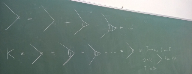
Here, first term is the two-point function in UV limit \& 


with boundary conditions 

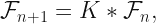
After this, we moved on to four-point functions, he termed them ‘ladder diagrams’.

This equation is
where 

The above equation he wrote in the eigenbasis as,

and started the program to evaluate its eigenvalues and eigenvectors.
He argued that 

 Motivated by this, he wrote the eigenvalue of
This is where he ended his lecture.
Madhusudhan Raman (IMSc) delivered the evening talk about basics of supersymmetry, in order to lay the groundwork for Victor’s talks on supersymmetric localization. He started with the Coleman-Mandula theorem which states that Poincare and internal symmetries cannot be combined an any way except trivially. Two interesting points came up during the discussion: (i) that this was a statement that was true under the assumption that the resulting theory has a non-trivial and analytic S-matrix, and (ii) that it doesn’t apply to lower-dimensional quantum field theories! Coleman and Mandula assumed that the group 

![[O_{a},O_{b}]=O_{a}O_{b}-(1)^{n_{a}n_{b}}O_{b}O_{a}](https://s0.wp.com/latex.php?latex=%5BO_%7Ba%7D%2CO_%7Bb%7D%5D%3DO_%7Ba%7DO_%7Bb%7D-%281%29%5E%7Bn_%7Ba%7Dn_%7Bb%7D%7DO_%7Bb%7DO_%7Ba%7D&bg=ffffff&fg=111111&s=2&c=20201002)
where,

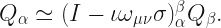
and he begin with definition of the supersymmetry algebra
![(a)~~~~~ [Q_{\alpha},M^{\mu\nu}]= \iota (\sigma^{\mu\nu})_{\alpha}^{\beta}Q_{\beta}](https://s0.wp.com/latex.php?latex=%28a%29%7E%7E%7E%7E%7E+%5BQ_%7B%5Calpha%7D%2CM%5E%7B%5Cmu%5Cnu%7D%5D%3D+%5Ciota+%28%5Csigma%5E%7B%5Cmu%5Cnu%7D%29_%7B%5Calpha%7D%5E%7B%5Cbeta%7DQ_%7B%5Cbeta%7D&bg=ffffff&fg=111111&s=0&c=20201002)
where, 
Then, he spoke about the effect of translations,
![(b)~~~~~~~~~~[Q_{\alpha},P^{\nu}]= 0.](https://s0.wp.com/latex.php?latex=%28b%29%7E%7E%7E%7E%7E%7E%7E%7E%7E%7E%5BQ_%7B%5Calpha%7D%2CP%5E%7B%5Cnu%7D%5D%3D+0.&bg=ffffff&fg=111111&s=2&c=20201002)
He explained by logical argument that the above commutator can be fixed in a simple way: let’s assume it transformed as
![[Q_{\alpha},P^{\mu}]= c(\sigma^{\mu})_{\alpha\dot{\alpha}}\bar{Q}^{\dot{\alpha}},](https://s0.wp.com/latex.php?latex=%5BQ_%7B%5Calpha%7D%2CP%5E%7B%5Cmu%7D%5D%3D+c%28%5Csigma%5E%7B%5Cmu%7D%29_%7B%5Calpha%5Cdot%7B%5Calpha%7D%7D%5Cbar%7BQ%7D%5E%7B%5Cdot%7B%5Calpha%7D%7D%2C&bg=ffffff&fg=111111&s=2&c=20201002)
then since the l.h.s. satisfies Jacobi’s identity with respect to 
![[P_{\mu},[P^{\mu},Q_{\beta}]]+cycl.= 0 ~ \text{which implies} \ c=0](https://s0.wp.com/latex.php?latex=%5BP_%7B%5Cmu%7D%2C%5BP%5E%7B%5Cmu%7D%2CQ_%7B%5Cbeta%7D%5D%5D%2Bcycl.%3D+0+%7E+%5Ctext%7Bwhich+implies%7D+%5C+c%3D0&bg=ffffff&fg=111111&s=2&c=20201002)
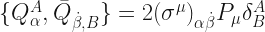
Next came the effects of the supercharges on each other,

using the same arguments we can show 

From the last relation it is clear that the supersymmetry transformation knows about the underlying space-time and also he explained why supersymmetry commutes with internal symmetries which are clear from this relation,
![[T_{a},Q_{\alpha}]=0.](https://s0.wp.com/latex.php?latex=%5BT_%7Ba%7D%2CQ_%7B%5Calpha%7D%5D%3D0.&bg=ffffff&fg=111111&s=2&c=20201002)
Then he explained the R-symmetry

It satisfies following relation
![[Q_{a},R] = Q_{a}](https://s0.wp.com/latex.php?latex=%5BQ_%7Ba%7D%2CR%5D+%3D+Q_%7Ba%7D&bg=ffffff&fg=111111&s=2&c=20201002)
![[\bar{Q}_{\dot{a}},R] =-\bar{Q}_{\dot{a}}](https://s0.wp.com/latex.php?latex=%5B%5Cbar%7BQ%7D_%7B%5Cdot%7Ba%7D%7D%2CR%5D+%3D-%5Cbar%7BQ%7D_%7B%5Cdot%7Ba%7D%7D&bg=ffffff&fg=111111&s=2&c=20201002)
so we observe that the supercharges are charged under R-symmetry. Then, he extend the SUSY algebra for 
where, A,B = 1, 2, 3, …, N.

where 
We know that Casmirs for Poincare algebra tell us how to label 1-particle states, i.e. we use the mass and spin/helicity.


then he explain what’s happen if we add SUSY (for example N=1) 


Then he gave an example for N=1 supersymmetry for massless particles, where we boost to the frame 

and we can define raising operator and lowering operators as

We know that for the massless particles helicity is good quantum number, as demonstrated by

In the last hour he spend the time to explain us a superspace 

Madhu stated that the idea of susysymmetry in superspace is lot like momentum in spacetime: it generates translations. We can give this idea a differential-operator meaning; just like momentum generates translations in space, supercharges generate translations in superspace!

How do superfields transform under infinitesimal coordinate changes generated by supercharges? It is simply
Eventually, one would like to write down actions in superspace. However, the general superfield has far too many fields, corresponding to a reducible representation of the SUSY algebra. In order to cut down the number of components, one needs to define derivative operators in superspace that anticommute with the supercharges. These can then be used to (a) effect constraints on superfields, that will reduce the number of fields, and (b) write down superactions in superspace. These differential operators look like

and
At the end, he explained that any action of the form

is — by construction! — SUSY invariant! The first term is known as the Kahler potential and the second is known as the superpotential. A short discussion of the statement of non-renormalization theorems followed, and that was where we concluded for the day.
