
On the final day of ST4 2018, we begin with a bunch of thank yous. We are deeply grateful to Prof. Sudhakar Panda, the Director of NISER, for signing off on letting us have the second edition of ST4 here. Our sincerest and most heartfelt thanks to Prof. Chethan Gowdigere for his pivotal support in the organisation of resources for ST4 2018, without which (it is safe to say) the organisers would have had to struggle quite a bit. Thanks also to the staff at NISER and the chai & coffee supplying bhaiyyas who made sure we never ran out of little things to eat or drink during lectures.
We thank all the attendees for participating in the democratic process of picking our speakers, and in doing so, also choosing the theme for ST4 2018. Thanks also for attending and having a good time, and for making our little meeting a success! Finally, thanks to the speakers who were all wonderful, solely responsible for making this ST4 a lot of fun, and were fully prepared with a nifty answer against our every worry in the classroom– we learnt a lot!
We hope to see you all again soon, at ST4 2019!
*******
Jahanur came back on the last day of ST4 2018 to compute the energy in the de Sitter spacetime, using notions of symplectic structures introduced by Aneesh the previous day.
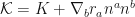
A brief review in possibly more familiar language follows. Consider the variation of the Langrangian 


where the last term is the total derivative whose integral variation we all like to set to zero on the boundary while deriving the equations of motion, which are denoted here by 


![[\delta_1,\delta_2]{\mathcal{L}}=0](https://s0.wp.com/latex.php?latex=%5B%5Cdelta_1%2C%5Cdelta_2%5D%7B%5Cmathcal%7BL%7D%7D%3D0&bg=ffffff&fg=111111&s=0&c=20201002)

then ![[\delta_1,\delta_2]{\mathcal{L}}=0\implies\nabla_\mu\omega^\mu=0](https://s0.wp.com/latex.php?latex=%5B%5Cdelta_1%2C%5Cdelta_2%5D%7B%5Cmathcal%7BL%7D%7D%3D0%5Cimplies%5Cnabla_%5Cmu%5Comega%5E%5Cmu%3D0&bg=ffffff&fg=111111&s=0&c=20201002)

or, using Gauss’ Theorem,

If the above summary didn’t resonate deeply with you, you can always visit Aneesh’s lecture notes.
Now, since Jahanur wants to compute the energy of the system, he considers a special class of hypersurfaces which are those generated by the the time-like Killing vector of the de Sitter metric 

This surface is defined by 


where,

For the energy computation we take, 


Diffeomorphisms are symmetries of any sane theory of gravity, and therefore the Lie derivatives of 

Anticipating algebraic convenience, Jahanur chooses to work with 


In usual practice (for flat spacetimes), according to the speaker, one gets by the above difficulty of computing the transverse traceless component by computing it only asymptotically. This is done by means of a propagator,

It turns out that,
That is, for flat space times, this difference in the two definitions does not matter as long as one is computing energy flux. Although, it may turn out to be important when one tries to compute angular momentum flux etc.
However, the above difference gives different notions of energy for de Sitter spacetimes. We compute this energy for 
![\begin{aligned} \omega^\eta &= \tfrac{1}{16\pi G}H^2\eta^2\left\lbrace\chi^{ij}\partial_\eta\left[ (T.\partial)\chi_{ij}\right]-(T.\partial)\chi_{ij}\partial_\eta\chi^{ij} \right\rbrace,\\ \omega^i &= \tfrac{1}{32\pi G}H^2\eta^2\delta^{ik}\left\lbrace\chi^{lm}\partial_m\left[(T.\partial)\chi_{kl}\right]-\tfrac{1}{2}\chi^{lm}\partial_k\left[(T.\partial)\chi_{lm}\right]-\left[(T.\partial)\chi^{lm}\right]\partial_m\chi_{kl}\right.\cr & \hspace{2.2cm}\left.+\tfrac{1}{2}\left[(T.\partial)\chi^{lm}\right]\partial_k\chi_{lm} \right\rbrace, \end{aligned}](https://s0.wp.com/latex.php?latex=%5Cbegin%7Baligned%7D++%5Comega%5E%5Ceta+%26%3D+%5Ctfrac%7B1%7D%7B16%5Cpi+G%7DH%5E2%5Ceta%5E2%5Cleft%5Clbrace%5Cchi%5E%7Bij%7D%5Cpartial_%5Ceta%5Cleft%5B+%28T.%5Cpartial%29%5Cchi_%7Bij%7D%5Cright%5D-%28T.%5Cpartial%29%5Cchi_%7Bij%7D%5Cpartial_%5Ceta%5Cchi%5E%7Bij%7D+%5Cright%5Crbrace%2C%5C%5C++%5Comega%5Ei+%26%3D+%5Ctfrac%7B1%7D%7B32%5Cpi+G%7DH%5E2%5Ceta%5E2%5Cdelta%5E%7Bik%7D%5Cleft%5Clbrace%5Cchi%5E%7Blm%7D%5Cpartial_m%5Cleft%5B%28T.%5Cpartial%29%5Cchi_%7Bkl%7D%5Cright%5D-%5Ctfrac%7B1%7D%7B2%7D%5Cchi%5E%7Blm%7D%5Cpartial_k%5Cleft%5B%28T.%5Cpartial%29%5Cchi_%7Blm%7D%5Cright%5D-%5Cleft%5B%28T.%5Cpartial%29%5Cchi%5E%7Blm%7D%5Cright%5D%5Cpartial_m%5Cchi_%7Bkl%7D%5Cright.%5Ccr++%26+%5Chspace%7B2.2cm%7D%5Cleft.%2B%5Ctfrac%7B1%7D%7B2%7D%5Cleft%5B%28T.%5Cpartial%29%5Cchi%5E%7Blm%7D%5Cright%5D%5Cpartial_k%5Cchi_%7Blm%7D+%5Cright%5Crbrace%2C++%5Cend%7Baligned%7D&bg=ffffff&fg=111111&s=0&c=20201002)
where the tt indices are suppressed and 

where the constant surface is 

where

Just to remind the reader,

which is the quadrupole moment in the de Sitter background.
***
We commenced after the break with Jahanur speaking to us about the ADM energy for de Sitter spacetimes,

where 

For the de Sitter metric,

we get 

Forget about the 
Now one has to juggle around with the (in)famous Gauss-Codazzi equations to rewrite 


where 


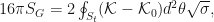
where the ADM mass is given by

Let’s look at some examples.
Computed for the flat Minkowski spacetime, this turns out to be,
![M_{ADM}\overset{flat}{=}\frac{1}{16\pi}\underset{S_t\rightarrow\infty}{lim} \oint \left[ D^j \gamma_{ij} - D_i (f^{kl}\gamma_{kl}) \right]s^i\sqrt{\sigma}d^2\theta,](https://s0.wp.com/latex.php?latex=M_%7BADM%7D%5Coverset%7Bflat%7D%7B%3D%7D%5Cfrac%7B1%7D%7B16%5Cpi%7D%5Cunderset%7BS_t%5Crightarrow%5Cinfty%7D%7Blim%7D+%5Coint+%5Cleft%5B+D%5Ej+%5Cgamma_%7Bij%7D+-+D_i+%28f%5E%7Bkl%7D%5Cgamma_%7Bkl%7D%29+%5Cright%5Ds%5Ei%5Csqrt%7B%5Csigma%7Dd%5E2%5Ctheta%2C&bg=ffffff&fg=111111&s=0&c=20201002)
where 

Consider the Schwarzchild spacetime:

where 


For de Sitter-Schwarzchild, this formula doesn’t work because 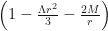

The ADM mass can also be derived from the construction of a Noether current. (An astute reader might ponder how one should use Noether’s theorem in a theory which has only gauge symmetries. In fact, Noether’s second theorem deals precisely with gauge symmetries! :P).

where 

![\epsilon=\int Q[t]-t.B](https://s0.wp.com/latex.php?latex=%5Cepsilon%3D%5Cint+Q%5Bt%5D-t.B&bg=ffffff&fg=111111&s=0&c=20201002)
Jahanur also discussed Kelly & Marolf‘s results on de Sitter charges on flat and hyperbolic slices (for 

There is yet another way to compute asymptotic charges. This one seems to be in vogue in the AdS/CFT community. Here, one computes first what is known as the Brown-York stress tensor for an action. This basically is the variation of the Einstein-Hilbert action w.r.t the boundary metric. One chooses an appropriate slicing: for negative curvature spaces, the slicing should be time-like whereas for positive curvature spaces, it must be space-like. Then one computes the charge along ones favourite symmetry of the boundary metric in the usual sense, from this Brown-York tensor. For the de Sitter case

where
![T_{ab}=\frac{2}{\sqrt{h}}\frac{\delta S}{\delta h^{ab}}=\frac{1}{8\pi G}\left[Kh^{ab}-K^{ab}+\frac{2}{l}h^{ab}+l R^{ab}-\frac{l}{2}R h^{ab} \right],](https://s0.wp.com/latex.php?latex=T_%7Bab%7D%3D%5Cfrac%7B2%7D%7B%5Csqrt%7Bh%7D%7D%5Cfrac%7B%5Cdelta+S%7D%7B%5Cdelta+h%5E%7Bab%7D%7D%3D%5Cfrac%7B1%7D%7B8%5Cpi+G%7D%5Cleft%5BKh%5E%7Bab%7D-K%5E%7Bab%7D%2B%5Cfrac%7B2%7D%7Bl%7Dh%5E%7Bab%7D%2Bl+R%5E%7Bab%7D-%5Cfrac%7Bl%7D%7B2%7DR+h%5E%7Bab%7D+%5Cright%5D%2C&bg=ffffff&fg=111111&s=0&c=20201002)
for the spacelike boundary surface.
Strominger et al., computed the charges for deSitter space. BUT! the asymptotic symmetry group of deSitter (according to Jahanur) is 

With this set of final comments, Jahanur bowed out. Phew, that was hectic and informative!
*******
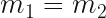
Chandan in his last lecture discussed open 
He then continued to discussed the renormalisability of this theory. By considering various beta functions for the couplings, he showed us how under renormalisation group flow the tree-level Lindblad conditions are protected even at one loop. He further mentioned that the Lindblad conditions are actually all loop exact! This strongly implies that
Markovianity of open
To calculate the beta functions for the quartic couplings at one loop, divergent contributions come from bubble diagrams. All the diagrams can be computed by evaluating just a single integral over loop momentum. This integral is hard to compute since space and time can not be treated on equal footing due to the structure of the integrand. With some hard work the integral can be performed to obtain all the beta functions till quartic order in the couplings, at one loop.
Chandan then discussed various non-local divergences that appear in the loop integrals for open quantum field theories by considering the case of
As an example consider the following amputated diagram (Fig 1) in 


The integral evaluates to,

where k is the external momentum. Notice that there is a 

The second example (Fig 2) to illustrate nonlocal divergence was for the Yukawa theory. Chandan considered the following self energy diagram for Dirac fermion.

Using the Passarino Veltman (PV) reduction, one can reduce the fermionic integral into a linear combination of two types (called the A and the B type) of scalar loop integrals. These integrals have non local divergences that prevail even when one sets 
And that was that. The organisers announced that ST4 2018 was at a close. Murmurs of the sort “okay, where do I sign up for ST4 2019” were heard and everyone happily left the classroom to go pack.
*******
Goodbye and thanks for following ST4 again this year.
See you again in 2019!
We will be back.
