Jahanur started off his second lecture with the aim of reviewing the Hamiltonian formalism of GR. The formalism was developed for a four-dimensional manifold  . The speaker announced at the start that he would not distinguish between the indices of
  and those of the metric over hypersurfaces with no timelike coordinate (which we shall shortly introduce) and thus, running over three possible values. This spacetime can be foliated using non-intersecting spacelike hypersurfaces
  with
with  , the coordinate along the timelike direction labelling these various hypersurfaces.
Defining the future directed normal as,
we can write the induced metric  on the spatial hypersurface as

and the raised projection tensor is,  . Note that
  is not the inverse metric. The speaker pointed out that all indices were raised/lowered with respect to , the four-dimensional metric on the full manifold. can be thought of as a projection tensor which projects out all geometric objects lying along
  . Following the construction of projection operators and studying their action on vectors and tensors, Jahanur proceeded to define covariant differentiation of a “purely spatial” vector field
  , restricted to the hypersurface . Predictably, it is essentially the projection of the four-dimensional its covariant derivative on the hypersurface i. e.,

For “purely spatial tensors,” an analog of the above equation with more  s sitting in front would be the appropriate definition of the covariant derivative on . For general tensors, with a non-zero projection along the normal, simply considering the covariant derivative and projecting it on won’t give you a purely spatial derivative: it will contain a piece proportional to the extrinsic curvature. The Riemann tensor for the hypersurface has no information about curvature of the embedding space
  . This is captured through the extrinsic curvature
  which is defined as,

which is symmetric in  . Through a series of manipulations and making use of the explicit form of , Jahanur eventually showed that the extrinsic curvature tensor is related to the Lie derivative of the induced metric along the normal vector, namely

After the coffee break, in an attempt to relate the Riemann tensor associated with in terms of the the Riemann tensor for , Jahanur ended up with the Gauss-Codazzi equations:

These are essentially integrability criteria which specify a particular spatial hypersurface through the data  in a higher dimensional ambient spacetime. These equations are also crucial in decomposing Einstein’s Equations in the Hamiltonian formulation which gives us the Hamiltonian constraint and the momentum constraint. They take the following form:

These equations capture the dynamics of a gravitational field at a particular snapshot of time  const.
The most natural question to ask after this point is what about the evolution of the  data as we go from one hypersurface to
  . It is to be noticed here that the Lie derivative along is not a natural time derivative thus necessitating the construction for
  . Starting with a one-form, which is normalized as
  . We define another vector
  , where
  is a spatial shift vector (thus,
  is dual to the
  vector). Physically, the vector is the congruence which takes a small patch from the hypersurface to another hypersurface infinitesimally away . The vector captures the shift in the coordinate points with respect to the normal. This spurred off an enthusiatic discussion amongst the audience regarding the special case when the vector is vanishing. Eventually, Jahanur wrote down the explicit form of
  in terms of derivatives of
  and
and  and their derivatives.
The formalism building was followed by the discussion of a special case where  , which is true if we make the choice
  . Over the last quarter of an hour, Jahanur described the ADM formalism starting from the Einstein-Hilbert action. He wrote down the Lagrangian density in terms of the hypersurface variables and gave a nice compact expression for the conjugate momenta on as,

In the last few minutes, he defined the electric part of the Weyl tensor in the context of de Sitter spaces with the promise that Aneesh would pick up from here and explain how it comes about in the next lecture. With hunger in our minds and stomach, we proceeded for lunch.
*******
After lunch, the inimitable Chandan Kumar Jana began his second lecture on open quantum systems, with the goal of introducing dissipation, defining notions of open quantum mechanics, and deriving the Lindblad equation. Historians of science will remember this evening as an especially entertaining one.
Before getting on with the days proceedings, Chandan started out by highlighting that the usual Schwinger-Keldysh contours are inadequate for computing certain correlators. Consider, as an example, the following correlator

with the time ordering  and
and  . A little fiddling around with contours will convince one that the last operator
  cannot be accommodated with the constraint
  ! This can be remedied in a straightforward manner: introduce another time-fold. In general, a
  -out of time ordered correlator (OTOC) is one with future turning points. For example, a
  -OTOC is the usual Schwinger-Keldysh contour, and a
  -OTOC is typically used in the computation of the chaos correlator.
We then moved on to business for the day. Recall from our example yesterday — the one with the particle attached to a spring that was in turn attached to a pendulum — that we were able to integrate out the position of the spring/oscillator,  , to write down an effective action for the position of the particle (tip of the pendulum) denoted by
  that looked (schematically) like this:
![\int \text{D}Q_R \text{D}Q_L \, \text{e}^{i S_{\text{SK}}[Q_R,Q_L]} \text{e}^{i \Phi[Q_R,Q_L]} \ ,](https://s0.wp.com/latex.php?latex=%5Cint+%5Ctext%7BD%7DQ_R+%5Ctext%7BD%7DQ_L+%5C%2C+%5Ctext%7Be%7D%5E%7Bi+S_%7B%5Ctext%7BSK%7D%7D%5BQ_R%2CQ_L%5D%7D+%5Ctext%7Be%7D%5E%7Bi+%5CPhi%5BQ_R%2CQ_L%5D%7D+%5C+%2C&bg=ffffff&fg=111111&s=0&c=20201002)
where  is the usual Schwinger-Keldysh action, and
  is the Feynman-Vernon influence functional, which has a complicated form and has information regarding the variable that has been integrated out. It is important to note, however, that the influence functional (written below in frequency space) itself has interesting structure:
![\Phi = \frac{1}{2\pi\hbar} \int_0^\infty \text{d}\nu \, \left[ \frac{\widetilde{Q}_L(\nu)[\widetilde{Q}_R(-\nu) - \widetilde{Q}_L(-\nu)]}{-m\left[ (\nu - i \epsilon)^2-\omega^2\right]} + \frac{\widetilde{Q}_R(-\nu)[\widetilde{Q}_R(\nu) - \widetilde{Q}_L(\nu)]}{-m\left[ (\nu + i \epsilon)^2-\omega^2\right]} \right].](https://s0.wp.com/latex.php?latex=%5CPhi+%3D+%5Cfrac%7B1%7D%7B2%5Cpi%5Chbar%7D+%5Cint_0%5E%5Cinfty+%5Ctext%7Bd%7D%5Cnu+%5C%2C+%5Cleft%5B+%5Cfrac%7B%5Cwidetilde%7BQ%7D_L%28%5Cnu%29%5B%5Cwidetilde%7BQ%7D_R%28-%5Cnu%29+-+%5Cwidetilde%7BQ%7D_L%28-%5Cnu%29%5D%7D%7B-m%5Cleft%5B+%28%5Cnu+-+i+%5Cepsilon%29%5E2-%5Comega%5E2%5Cright%5D%7D+%2B+%5Cfrac%7B%5Cwidetilde%7BQ%7D_R%28-%5Cnu%29%5B%5Cwidetilde%7BQ%7D_R%28%5Cnu%29+-+%5Cwidetilde%7BQ%7D_L%28%5Cnu%29%5D%7D%7B-m%5Cleft%5B+%28%5Cnu+%2B+i+%5Cepsilon%29%5E2-%5Comega%5E2%5Cright%5D%7D+%5Cright%5D.&bg=ffffff&fg=111111&s=0&c=20201002)
The quantity  , defined as,
![\frac{1}{i\nu Z_\nu} = \frac{1}{-m\left[ (\nu - i \epsilon)^2-\omega^2\right]} \ ,](https://s0.wp.com/latex.php?latex=%5Cfrac%7B1%7D%7Bi%5Cnu+Z_%5Cnu%7D+%3D+%5Cfrac%7B1%7D%7B-m%5Cleft%5B+%28%5Cnu+-+i+%5Cepsilon%29%5E2-%5Comega%5E2%5Cright%5D%7D+%5C+%2C&bg=ffffff&fg=111111&s=0&c=20201002)
is an impedance, Chandan said, and the room fell silent. “What the hell did impedance have to do with anything?,” some members of the audience members wondered. Then Chandan muttered the words “LCR circuit,” and all hell broke loose.
Perhaps some explanation is in order: although it is actually not at all difficult to work out, the mention of certain topics — usually those from undergraduate textbooks — like Carnot engines, for example, send the otherwise respectable graduate student into a panic-induced fury. This was one of those times. We had, however, the dulcet tones of Prashant Kocherlakota (TIFR), who helpfully reminded the audience what an LCR circuit is. Basically, if a circuit has an inductor with inductance  , a capacitor with capacitance
  , and a resistance with resistance
  , all in series, the equation obeyed by the charge
  as a function of time is,

where  is the potential and plays the role of the forcing term in an LCR circuit. The above equation is simply solved in the frequency domain by,

which contains essentially the Fourier transform of the Green’s function. Basically, if the Green’s function has an imaginary part, you’re going to have dissipation. In the case of the particle , it’s going to give some of its energy to the oscillator that we’d integrated out, and in the case of an LCR circuit, it is going to leak out because current flowing through a resistor will heat it up.
On to open quantum mechanics. We assume that the Hilbert space of our total system splits into two parts: that of the subsystem we’re interested in  and that of the environment
  . The strategy of our computation will be to start with a density matrix
  ,
,

where  is not a density matrix; rather, it keeps track of all correlations between the system and its environment, a sort of correction term. We want to start with this state and evolve in time to
  , then trace out the environmental degrees of freedom. This is a bit involved, so we’ll save the details for the notes and state the end result here:

where  are called Kraus operators, and are essentially matrix elements of the global unitary time evolution operator in some environmental basis. Chandan then stated a couple of theorems without proof:
- if the initial -state is pure, then is zero identically, and
- the above equation for
 can re-written by redefining the Kraus operators to depend on the initial -state, and this has the effect of absorbing the
  .
.
We’ll end our discussion of Chandan’s lecture for today by discussing a particularly thorny issue regarding the manner in which quantum systems evolve. Theorem 1 above states that if we start off with a pure state, then is identically zero. Now consider time-evolving a system from  to
to  in two different ways: first, directly; and second, by stopping off at first. Define a universal dynamical map (UDM) as one where the Kraus operator doesn’t depend on the initial -state, and a Markovian evolution as one where time-evolution is derived by composing UDMs. As we have seen, however, this can’t work because in the time between and , the system will have developed correlations, and consequently will not be a pure state.
In general, open quantum system evolution is not Markovian. However, in those situations where doesn’t affect the dynamics appreciably, i.e., when the time scale for decay of system-environment correlations is smaller than the time scale on which we are interested in tracking (or probing) the evolution of the system, we can make a Markovian approximation. Assuming this, we can derive a linear time-evolution equation called the Lindblad equation, whose details we will explore in greater detail tomorrow.
*******
The evening talk of the day was delivered by Prashant Kocherlakota (TIFR, Mumbai) on the time evolution of spins in a gravitational field. The aim of the lecture was to discuss how one defines angular momentum in general relativity, what the notion of intrinsic angular momentum is, how it ‘couples to a stationary gravitational field’ and whether one can measure this coupling, which turns out to be linked to the vorticity in the spacetime, by local experiments or by experiments conducted on Earth. The lecture became very catchy, mainly because the topics he covered appeared to be essential for a comprehensive understanding of some aspects of stationary spacetime geometries like frame-dragging and vorticity.
The speaker started with a brief explanation of how one deals with angular momentum in Newtonian classical mechanics and went on to generalize the same for curved space-time. He assured us that this was all lifted from box 5.6 of Misner, Thorne & Wheeler’s Gravitation.
Before moving to the derivation of the covariant equation of motion for a spinning object, he argued that the intrinsic spin of an object can only be defined with respect to the local rest frame of the body initially. This mathematically is given as,

where  is just the inner product, is the spin four-vector and
  is the four-velocity of the spinning object along its world-line. Here, intrinsic spin is meant to describe either the <expectation of the> polarization vector of a quantum particle or the intrinsic angular momentum of a rigid body like a gyroscope or a pulsar(!?), he continued. Under the assumption that no external force acts upon the spinning object, and that its quadrupole moment doesn’t couple with inhomogeneities of the gravitational field, one naturally writes in its rest frame,

which he showed becomes covariantly,

where  is the acceleration.
Prashant then (preemptively) defined the Fermi derivative of a vector along a world line , with a tangent vector  as,
as,

He went on to discuss how the notion of Fermi-transport is a useful tool in the study of spinning objects, in general relativity. The equation of motion for the spin vector reduces to the statement that the spin vector is Fermi transported along its path. i.e.,

The Fermi derivative has the property that it also Fermi transports along itself. Further, since one has  and both vectors are Fermi transported (along ), the two vectors remain orthogonal all along . This implies that remains in the directions perpendicular to always and one may introduce an orthonormal spatial triad that is also orthogonal to , in which to project and its equation of motion to simplify matters.
The next discussion was on the “Frenet-Serret frame,” which happens to be just such a frame. To understand the Frenet-Serret frame clearly, Prashant restricted to defining it along an arbitrary curve  in
in ![(\mathbb{R}^3, diag[1,1,1])](https://s0.wp.com/latex.php?latex=%28%5Cmathbb%7BR%7D%5E3%2C+diag%5B1%2C1%2C1%5D%29&bg=ffffff&fg=111111&s=0&c=20201002) . The goal was to derive the Frenet-Serret equations, which describe how the triad fields evolve along , and to show how they involve the inherent properties of the curve like its curvature
. The goal was to derive the Frenet-Serret equations, which describe how the triad fields evolve along , and to show how they involve the inherent properties of the curve like its curvature  and torsion
  . The tangent, normal, and binormal unit vectors, denoted by
  ,
,  , and
, and  , form an orthonormal basis and the Frenet-Serret equations can be written in matrix form as,

Prashant then showed that the equation of motion for the spin three vector in the Frenet-Serret frame becomes just,
 ,
,
where  is related to the vorticity two-form,
  (which vanishes in static spacetimes but is non-zero in stationary spacetimes) and the above equation is written in the FS spatial triad. This just means that a spin vector just appears to precesses in a stationary spacetime!
Prashant concluded his talk by briefly talking about some results of projects he was part of which were related to the precession of gyroscopes on Killing orbits of the Kerr spacetime. In such cases, is simply the normalised vorticity of the Killing congruence and the following table summarises some results,
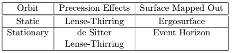
He also discussed how these pertained to local experiments. We were too tired and hungry to listen to Prashant prattle on about how he’s applying this stuff to pulsars, and reading the temperature of the room correctly, he obliged us by letting us go.


![[\delta_1,\delta_2]{\mathcal{L}}=0](https://s0.wp.com/latex.php?latex=%5B%5Cdelta_1%2C%5Cdelta_2%5D%7B%5Cmathcal%7BL%7D%7D%3D0&bg=ffffff&fg=111111&s=0&c=20201002)

![[\delta_1,\delta_2]{\mathcal{L}}=0\implies\nabla_\mu\omega^\mu=0](https://s0.wp.com/latex.php?latex=%5B%5Cdelta_1%2C%5Cdelta_2%5D%7B%5Cmathcal%7BL%7D%7D%3D0%5Cimplies%5Cnabla_%5Cmu%5Comega%5E%5Cmu%3D0&bg=ffffff&fg=111111&s=0&c=20201002)


![\begin{aligned} \omega^\eta &= \tfrac{1}{16\pi G}H^2\eta^2\left\lbrace\chi^{ij}\partial_\eta\left[ (T.\partial)\chi_{ij}\right]-(T.\partial)\chi_{ij}\partial_\eta\chi^{ij} \right\rbrace,\\ \omega^i &= \tfrac{1}{32\pi G}H^2\eta^2\delta^{ik}\left\lbrace\chi^{lm}\partial_m\left[(T.\partial)\chi_{kl}\right]-\tfrac{1}{2}\chi^{lm}\partial_k\left[(T.\partial)\chi_{lm}\right]-\left[(T.\partial)\chi^{lm}\right]\partial_m\chi_{kl}\right.\cr & \hspace{2.2cm}\left.+\tfrac{1}{2}\left[(T.\partial)\chi^{lm}\right]\partial_k\chi_{lm} \right\rbrace, \end{aligned}](https://s0.wp.com/latex.php?latex=%5Cbegin%7Baligned%7D++%5Comega%5E%5Ceta+%26%3D+%5Ctfrac%7B1%7D%7B16%5Cpi+G%7DH%5E2%5Ceta%5E2%5Cleft%5Clbrace%5Cchi%5E%7Bij%7D%5Cpartial_%5Ceta%5Cleft%5B+%28T.%5Cpartial%29%5Cchi_%7Bij%7D%5Cright%5D-%28T.%5Cpartial%29%5Cchi_%7Bij%7D%5Cpartial_%5Ceta%5Cchi%5E%7Bij%7D+%5Cright%5Crbrace%2C%5C%5C++%5Comega%5Ei+%26%3D+%5Ctfrac%7B1%7D%7B32%5Cpi+G%7DH%5E2%5Ceta%5E2%5Cdelta%5E%7Bik%7D%5Cleft%5Clbrace%5Cchi%5E%7Blm%7D%5Cpartial_m%5Cleft%5B%28T.%5Cpartial%29%5Cchi_%7Bkl%7D%5Cright%5D-%5Ctfrac%7B1%7D%7B2%7D%5Cchi%5E%7Blm%7D%5Cpartial_k%5Cleft%5B%28T.%5Cpartial%29%5Cchi_%7Blm%7D%5Cright%5D-%5Cleft%5B%28T.%5Cpartial%29%5Cchi%5E%7Blm%7D%5Cright%5D%5Cpartial_m%5Cchi_%7Bkl%7D%5Cright.%5Ccr++%26+%5Chspace%7B2.2cm%7D%5Cleft.%2B%5Ctfrac%7B1%7D%7B2%7D%5Cleft%5B%28T.%5Cpartial%29%5Cchi%5E%7Blm%7D%5Cright%5D%5Cpartial_k%5Cchi_%7Blm%7D+%5Cright%5Crbrace%2C++%5Cend%7Baligned%7D&bg=ffffff&fg=111111&s=0&c=20201002)


![M_{ADM}\overset{flat}{=}\frac{1}{16\pi}\underset{S_t\rightarrow\infty}{lim} \oint \left[ D^j \gamma_{ij} - D_i (f^{kl}\gamma_{kl}) \right]s^i\sqrt{\sigma}d^2\theta,](https://s0.wp.com/latex.php?latex=M_%7BADM%7D%5Coverset%7Bflat%7D%7B%3D%7D%5Cfrac%7B1%7D%7B16%5Cpi%7D%5Cunderset%7BS_t%5Crightarrow%5Cinfty%7D%7Blim%7D+%5Coint+%5Cleft%5B+D%5Ej+%5Cgamma_%7Bij%7D+-+D_i+%28f%5E%7Bkl%7D%5Cgamma_%7Bkl%7D%29+%5Cright%5Ds%5Ei%5Csqrt%7B%5Csigma%7Dd%5E2%5Ctheta%2C&bg=ffffff&fg=111111&s=0&c=20201002)


![\epsilon=\int Q[t]-t.B](https://s0.wp.com/latex.php?latex=%5Cepsilon%3D%5Cint+Q%5Bt%5D-t.B&bg=ffffff&fg=111111&s=0&c=20201002)


![T_{ab}=\frac{2}{\sqrt{h}}\frac{\delta S}{\delta h^{ab}}=\frac{1}{8\pi G}\left[Kh^{ab}-K^{ab}+\frac{2}{l}h^{ab}+l R^{ab}-\frac{l}{2}R h^{ab} \right],](https://s0.wp.com/latex.php?latex=T_%7Bab%7D%3D%5Cfrac%7B2%7D%7B%5Csqrt%7Bh%7D%7D%5Cfrac%7B%5Cdelta+S%7D%7B%5Cdelta+h%5E%7Bab%7D%7D%3D%5Cfrac%7B1%7D%7B8%5Cpi+G%7D%5Cleft%5BKh%5E%7Bab%7D-K%5E%7Bab%7D%2B%5Cfrac%7B2%7D%7Bl%7Dh%5E%7Bab%7D%2Bl+R%5E%7Bab%7D-%5Cfrac%7Bl%7D%7B2%7DR+h%5E%7Bab%7D+%5Cright%5D%2C&bg=ffffff&fg=111111&s=0&c=20201002)


 , as an initial condition for classical evolution and therefore the phase space is also the space of classical solutions.
 -form is a fully antisymmetric tensor with
 denotes wedge product which is just a fancy way of saying that the different
  s anticommute with each other.
 -form. The reason forms are interesting is that they are the natural objects that are integrated on
  ‘s point in the same direction; this is why the volume of a parallelopiped is the fully anti-symmetrised product of its three ‘basis’ vectors.
 is a way to label both positions and momenta with the same variable, so that
  . The Poisson brackets are given by the inverse of the symplectic form,
 . These can be thought of as flows on phase space, by identifying the components
  (where this derivative need not be with actual time, just come continuous parameter that parametrises the amount of flow). There are two types of flows on phase space: those that can be written as

 dimensions, he began with the space
  of all ‘kinematically allowed’ metrics on a manifold
  , where by ‘kinematically allowed’ he meant metrics one wouldn’t be devastated to find as solutions to one’s equations of motion. He then explained the rather involved process of defining the symplectic form as a two-form on the manifold
  and the completely antisymmetric
 are the Einstein equations, and the second term is the familiar boundary term one always finds (and willy-nilly sets to 0) while integrating by parts to find equations of motion from a Lagrangian — in this case, it is known as the presymplectic potential. The name is analogous to a gauge potential, since
  and
and  are indistinguishable — there is a gauge-invariance in
  -form,
 . Then, we got the real pre-symplectic form. This was still not the true phase space, since two diffeomorphism-related metrics are two different points in
  in the symplectic form to get the generator of infinitesimal transformations of that form, and then try to integrate it to find the Noether charge. He showed how this worked for the specific example of the charge conjugate to the translations in conformal time that Jahanur had indicated would be central to understanding gravitational waves in de Sitter.

 number of orthonormal basis matrices
  . We then took a particular basis set in which
  and all other basis matrices are traceless (For eg.
  form a basis of
  complex matrices). We then defined some new variables in terms of these basis matrices. The condition that the evolution preserves the trace, was the final ingredient to derive the Lindblad equation.
![\frac{d\rho}{dt}=-i[H,\rho]+\sum_{j,k}a_{jk}[F_j\rho F_k^\dagger-\frac{1}{2}\{F_k^\dagger F_j,\rho\}],](https://s0.wp.com/latex.php?latex=%5Cfrac%7Bd%5Crho%7D%7Bdt%7D%3D-i%5BH%2C%5Crho%5D%2B%5Csum_%7Bj%2Ck%7Da_%7Bjk%7D%5BF_j%5Crho+F_k%5E%5Cdagger-%5Cfrac%7B1%7D%7B2%7D%5C%7BF_k%5E%5Cdagger+F_j%2C%5Crho%5C%7D%5D%2C&bg=ffffff&fg=111111&s=0&c=20201002)
 was shown to be a positive semi definite matrix. Curious readers can access the
 ![Trace([H,\rho])=0](https://s0.wp.com/latex.php?latex=Trace%28%5BH%2C%5Crho%5D%29%3D0&bg=ffffff&fg=111111&s=0&c=20201002) . The fact that commutator has zero trace while true for finite dimensional systems (as
. The fact that commutator has zero trace while true for finite dimensional systems (as  ), is not true for infinite dimensional systems in general. We then wondered if this told us that Lindblad equation applied only to a finite dimensional Hilbert space, or if the particular trace we evaluated would still be zero by some nice properties of the Hamiltonian and the density operator. In any case, the audience, who struggled to comprehend the jump to the Lindblad equation from the assumptions on the second day, were happier when this outline was presented and were ready for new stuff.
 . Define
  , then the unitarity condition can be written as,
 are some basis vectors. Chandan told us that (according to Veltmann), this should be true diagram by diagram. It was pointed out by members in the audience that (if we trust Veltmann) in a
  theory, if we apply this to the four point function on the left side, we obtain product of three point vertices on the right side which are zero. Hence, in this case, the condition reduces to the imaginary part of
  being zero. Thus
  ,
,  and
and  . This was recast as the largest time equation for general diagrams. We used the largest time equation to “cut” various diagrams, in the sense that the RHS,
  and
and  are on-shell. Therefore, the largest time equation can be used to make the internal lines (off-shell) on the left side to external lines (on-shell) in the diagrams appearing on the right side, which can also be seen as cutting the diagram on the left in various ways to convert internal lines to external lines.
 , then the cutting equation reduces to the statement that all correlation functions with the difference field are zero.
 to zero, barring the identity operator. Now, he argued, we can compactify one of the direction and study the CFT on a
  , where the length of the circle can be identified as a temperature. But introducing a length scale in the system will cost us: we will now have nonzero one-point functions for arbitrary primary operators, in principle. Although, because of the translational invariance, one-point functions of any descendents will still vanish. The one point function of a scalar primary operator is given by,
 , he says. Using OPE, a two-point function can be written as,
 and
and  .
.  is the full conformal block for a thermal two point function.
 is not fixed, one cannot directly apply numerical bootstrap techniques. Rather, we will derive a powerful inversion formula which will enable the use of the KMS condition to do large spin analysis.
 and the two-point function can be written as,
 have simple poles in the space of
 to find the expression of
  invariance allows us to fix all the coordinates along a line and measure distance only in that direction. Therefore, we use coordinates
  and
and  . For simplicity, Kausik showed the derivation of inversion formula in 2d, but similar reasoning follows through in higher dimension.
 and
and  . So, in the Euclidean version the formula for
 ,
,  and
and  in the complex
  plane. Then, Kausik explained that the
  contour can be deformed around the bruch cuts. For our purpose, we deform the contour for
  towards the origin and for
  , we deform the contour towards the infinity. There is a symmetry under
  , which relates these deformations.
 therefore obtaining the Lorentzian inversion formula, starting from a Euclidean formula.
 type model in large
  field involved gives the thermal mass
  . Numerically, the thermal mass has been solved for. In the finite temperature regime, the correlators of energy momentum tensors are not studied extensively. It will help to explore the AdS side and to also find transport coefficients.
 and
and  in this frame. A detailed analysis of these Weyl scalars shows that
  falls off as
  , where
  is understood as affine parameter along null direction. As
  , it can be used to characterize the gravitational radiation.
 ,
,  , here
  and
and  are the coordinate indices which are raised and lowered by
  and
and  and
and  are the frame indices which are lowered and raised by
  . We can think of
  as a four vector defined at each point of space time. i.e,
  with
with  being real and null and
  being null and complex. By defining
  along the outgoing null direction and
  along the incoming null direction we can choose a non orthogonal basis.
 vector and it leaves
  invariant. This can be shown by using the antisymmetry property of the Weyl tensor
  . On the other hand the second class of transformation leaves the
  vector unchanged as a result
  becomes invariant. This type of rotations are important over the others because it leaves
  `origin-independent’ for asymptotically flat space-time. The concept of radiation is ‘less invariant’ in cases when
  does not have a null character. Namely the radiative component
  can be visualized as a hyperboloid in 5 dimensional Minkowski spacetime,
![ds^2= -dt^2+H^{-2} \cosh^{2}{Ht}{[d \chi^{2}+sin^{2} \chi(d \theta^2+sin^2 \theta d\phi^2)]}](https://s0.wp.com/latex.php?latex=ds%5E2%3D+-dt%5E2%2BH%5E%7B-2%7D+%5Ccosh%5E%7B2%7D%7BHt%7D%7B%5Bd+%5Cchi%5E%7B2%7D%2Bsin%5E%7B2%7D+%5Cchi%28d+%5Ctheta%5E2%2Bsin%5E2+%5Ctheta+d%5Cphi%5E2%29%5D%7D&bg=ffffff&fg=111111&s=0&c=20201002) .
. and
and  . Gravitational source is at the origin so it is sufficient to restrict to the future Poincare patch. The metric of future Poincare patch in
  coordinates is conformally flat,
  . We make a gauge choice
  which will decouple the linearized equations and for further simplification the rescaled tensor
  with
with  is used in the rest of the calculations. After exhausting all gauge freedoms we solved the non-zero components of field using Green’s function technique.

 where
where  is the free Hamiltonian, and
  is the interacting Hamiltonian. The interacting ground state is
  , and let the ground state of the corresponding free theory be
  . By considering the time to be complex (!), we can derive an expression for the interacting ground state in terms of the free ground state.

 .We then need to use perturbation theory to compute the left hand side order by order in the coupling constant. However, we will need to assume for this computation, that the in vacuum and the out vacuum are related by a phase. However, this is not true in general for quantum field theories. For field theories in curved spacetime, for theories with sources, the in vacuum maybe a linear combination of the out states. Therefore to compute any such correlation function in these theories we will need to sum over all the out states. This makes the computation harder in such situations, Schwinger Keldysh formalism provides a prescription to directly calculate this sum without needing to know the out states.
 which evolves a basis wave function
  .
.
![K(x_2,t_2;x_1,t_1)=\int [DX]e^{iS[x]}](https://s0.wp.com/latex.php?latex=K%28x_2%2Ct_2%3Bx_1%2Ct_1%29%3D%5Cint+%5BDX%5De%5E%7BiS%5Bx%5D%7D&bg=ffffff&fg=111111&s=0&c=20201002) . Then the probability of the state
. Then the probability of the state  is given by
 then we will have on the right hand side,
![\rho_{ini}(x_1,x_1^\prime)\delta(x_2-x_2^\prime)K(x_2,x_1)K^*(x_2^\prime,x_1^\prime)=\int_{\rho_{ini}}^{x_2=x_2^\prime|_{t_2}}[DX][DX^\prime]e^{iS[X]-iS[X\prime]}](https://s0.wp.com/latex.php?latex=%5Crho_%7Bini%7D%28x_1%2Cx_1%5E%5Cprime%29%5Cdelta%28x_2-x_2%5E%5Cprime%29K%28x_2%2Cx_1%29K%5E%2A%28x_2%5E%5Cprime%2Cx_1%5E%5Cprime%29%3D%5Cint_%7B%5Crho_%7Bini%7D%7D%5E%7Bx_2%3Dx_2%5E%5Cprime%7C_%7Bt_2%7D%7D%5BDX%5D%5BDX%5E%5Cprime%5De%5E%7BiS%5BX%5D-iS%5BX%5Cprime%5D%7D+&bg=ffffff&fg=111111&s=0&c=20201002)
 is the initial density matrix. Schwinger-Keldysh formalism is in fact based on such a path integral. We can see that in this path integral,
  and then
  is evolved back in time.
 in a density matrix
  , we get
![\langle O(t) \rangle = Tr[O(t)\rho]=\sum_i \lambda_i \langle \alpha_i|U^\dagger(t_0)O_I(t)U(t,0)|\alpha_i\rangle](https://s0.wp.com/latex.php?latex=%5Clangle+O%28t%29+%5Crangle+%3D+Tr%5BO%28t%29%5Crho%5D%3D%5Csum_i+%5Clambda_i+%5Clangle+%5Calpha_i%7CU%5E%5Cdagger%28t_0%29O_I%28t%29U%28t%2C0%29%7C%5Calpha_i%5Crangle+&bg=ffffff&fg=111111&s=0&c=20201002)
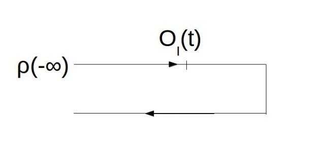
![\langle O(t) \rangle = Tr[U(-\infty,\infty)U(\infty,t)O_I(t)U(t,-\infty)\rho(-\infty)]](https://s0.wp.com/latex.php?latex=%5Clangle+O%28t%29+%5Crangle+%3D+Tr%5BU%28-%5Cinfty%2C%5Cinfty%29U%28%5Cinfty%2Ct%29O_I%28t%29U%28t%2C-%5Cinfty%29%5Crho%28-%5Cinfty%29%5D+&bg=ffffff&fg=111111&s=0&c=20201002)
 upto time
  at time
  to
to  and then again to
  . Thus, when computing one-point function in density matrices, we can obtain a way to do this via a closed time contour where we evolve forward in time and then backward evolve from infinity. We then saw how we can compute out of time ordered correlators also in this description, which are interesting in certain physical systems.
 and
and  , with L and R denoting the reverse and forward evolving contours. Operators along R(L) are (anti-)time ordered. We then considered the possible Green’s functions in this prescription,
  and
and  number of external particles if momentum of any massless particle becomes infinitesimally small then the amplitude can be expressed as a product form of soft factor, which depends on momenta and polarizations of the scattered particles, and amplitude of
 and the terms in the parentheses are soft factors. The soft factorization beyond leading term were discovered by Cachazo and Strominger. Based on the work by Chakrabarty, Kashyap, Sahoo, Sen and Verma and Sen, Laddha; Arpan mentioned that the soft factors,
  and
and  are universal for any gravitational theory and any process and are valid to all loop levels in perturbative S-matrix provided the dimension of spacetime is greater than or equal to five. In
  due to the infrared divergence issues of S-matrix the expressions of the soft factors are valid to tree level only.
 perturbative expansions.
  , which is topologically
  .
.  can be mapped to complex plane whose coordinates are
  . It turns out that
  and
and  are the free radiative data depending on
  and correspond to the two polarization degrees of freedom of graviton in four dimensions. Using Einstein’s equations all other metric perturbations can be solved in terms of these two data. Now the question is what are transformations that preserve the above form of the metric. These transformations are generated by supertranslations and six
  generators. Supertranslations are angle dependent translations at every point on
 . Arpan explained that BMS group was extended to generalized BMS group by Alok and Miguel and where
  which contains superroation vector fields given by
 and
and  are arbitrary vector field on
  , where
  is the linearized metric perturbation. Hence, the quantization of
  , naturally gives a quantization of free data, and hence quantization of charges. Hence, one can write the Ward identity,
![\langle \text{out}| \left[Q, S\right]|\text{in}\rangle = 0 .](https://s0.wp.com/latex.php?latex=%5Clangle+%5Ctext%7Bout%7D%7C+%5Cleft%5BQ%2C+S%5Cright%5D%7C%5Ctext%7Bin%7D%5Crangle+%3D+0+.&bg=ffffff&fg=111111&s=0&c=20201002)
 , to define symmetry of scattering process a matching condition called antipodal identifications is needed which relate free data at
  and
and  antipodally on
 ![\left[Q_{f},\left[Q_{V}, S\right]\right]](https://s0.wp.com/latex.php?latex=%5Cleft%5BQ_%7Bf%7D%2C%5Cleft%5BQ_%7BV%7D%2C+S%5Cright%5D%5Cright%5D&bg=ffffff&fg=111111&s=0&c=20201002) evaluated between in and out scattering states produce one of the consecutive double soft graviton theorem.
evaluated between in and out scattering states produce one of the consecutive double soft graviton theorem. ![\left[Q_{V},\left[Q_{f}, S\right]\right]](https://s0.wp.com/latex.php?latex=%5Cleft%5BQ_%7BV%7D%2C%5Cleft%5BQ_%7Bf%7D%2C+S%5Cright%5D%5Cright%5D&bg=ffffff&fg=111111&s=0&c=20201002) though formally produce the other consecutive double soft theorem, there are some mathematical subtleties about it, as the action of supertranslation charges on the superrotated vaccum is not well defined. Arpan referred us to their paper to figure out details of the story.
though formally produce the other consecutive double soft theorem, there are some mathematical subtleties about it, as the action of supertranslation charges on the superrotated vaccum is not well defined. Arpan referred us to their paper to figure out details of the story. and
and  , which are called the conformal data. It can also fix four-point correlators up to some arbitrary functions of conformal cross ratios. Then he went on to define what are known as conformal blocks. For this purpose, he first defined conformal partial waves (CPW).
 are conformal partial waves. Conformal blocks are functions of conformal cross ratios and related to the CPWs through a scale factor. For 2D CFTs, using conformal invariance he showed that one can set (
 ), which simplifies the expressions of the CPWs and the CBs a lot. Pinaki also mentioned the integral representation of the CBs given by
  of the CFT is very large (
 ) and both the heavy (
 ) and the light operators (
 ) in the theory scale as the central charge (

 . In this way, one can show that arbitrary
  -point (
 – point) blocks with two heavy and
  (or
(or  ) light operators factorize into
  numbers of H-L-L-H blocks (
 numbers of H-L-L-H blocks and one H-L-H block). This result has nice interpretation in terms of bulk geodesic diagrams in
  conical defect geometry (since
  means
means  and one can think the dual gravity theory as being classical).
 ) correlator which gives entanglement entropy for
  disjoint intervals in exited state. The same quantity can also be reproduced from the bulk geodesic picture.
 ) at finite temperature
  . He defined torus 1-point function for the primary operator
  with dimension
  and with torus modular parameter
 behaviour with
  behaviour.
![\overline{\langle E|{\cal O}|E\rangle} \approx N \langle \chi|{\cal O}|\chi\rangle \left(E - \frac{c}{12} \right)^{\frac{E_{\cal O}}{2}}~\text{exp}\left[- \frac{\pi c}{3} \bigg(1 - \sqrt{1 - \frac{12 E_{\chi}}{c}}\bigg) \sqrt{\frac{12 E}{c}-1} \, \right],](https://s0.wp.com/latex.php?latex=%5Coverline%7B%5Clangle+E%7C%7B%5Ccal+O%7D%7CE%5Crangle%7D+%5Capprox+N+%5Clangle+%5Cchi%7C%7B%5Ccal+O%7D%7C%5Cchi%5Crangle+%5Cleft%28E+-+%5Cfrac%7Bc%7D%7B12%7D+%5Cright%29%5E%7B%5Cfrac%7BE_%7B%5Ccal+O%7D%7D%7B2%7D%7D%7E%5Ctext%7Bexp%7D%5Cleft%5B-+%5Cfrac%7B%5Cpi+c%7D%7B3%7D+%5Cbigg%281+-+%5Csqrt%7B1+-+%5Cfrac%7B12+E_%7B%5Cchi%7D%7D%7Bc%7D%7D%5Cbigg%29+%5Csqrt%7B%5Cfrac%7B12+E%7D%7Bc%7D-1%7D+%5C%2C+%5Cright%5D%2C&bg=ffffff&fg=111111&s=0&c=20201002)
 is the lowest energy state with which
  and
and  :
:![\overline{\langle E|{\cal O}|E\rangle}\approx \tilde{N}_{\cal O}\langle \chi|{\cal O}|\chi\rangle\left(\frac{12 E}{c}-1\right)^{\frac{E_{\cal O}}{2}}~\text{exp}\left[-2\pi E_{\chi}\sqrt{\frac{12 E}{c}-1}\right]](https://s0.wp.com/latex.php?latex=%5Coverline%7B%5Clangle+E%7C%7B%5Ccal+O%7D%7CE%5Crangle%7D%5Capprox+%5Ctilde%7BN%7D_%7B%5Ccal+O%7D%5Clangle+%5Cchi%7C%7B%5Ccal+O%7D%7C%5Cchi%5Crangle%5Cleft%28%5Cfrac%7B12+E%7D%7Bc%7D-1%5Cright%29%5E%7B%5Cfrac%7BE_%7B%5Ccal+O%7D%7D%7B2%7D%7D%7E%5Ctext%7Bexp%7D%5Cleft%5B-2%5Cpi+E_%7B%5Cchi%7D%5Csqrt%7B%5Cfrac%7B12+E%7D%7Bc%7D-1%7D%5Cright%5D&bg=ffffff&fg=111111&s=0&c=20201002)
 are light fields in the bulk, which is a BTZ black hole for large enough
  . And
. And  can be reproduced from the following bulk geodesic picture.
 and
and  :
: and can thus not be thought of a perturbative field. Therefore, one should think of
 need to have same action on all the states in the code subspace. That is, as long as an observer is restricted to (sufficiently) low energy experiments, he/she can not differentiate these two HKLL representations of the bulk field. The code subspace can hence be thought of as an effective field theory subspace. “In this lecture, we will see how to define a general state in the code subspace and from there we derive the
  is a set of operators that close under addition or multiplication. From now on, we consider algebras that are defined in the space of
  matrices. Also, we deal with algebras that include the identity element and that are closed under Hermitian conjugation (i.e., if
  ). Next, we define the notion of commutant of an algebra. For any algebra
  is an algebra of all operators that commute with all the elements of
  is called the centre of
  is an algebra of all operators on
  such that
 ![Tr[\rho] =1](https://s0.wp.com/latex.php?latex=Tr%5B%5Crho%5D+%3D1&bg=ffffff&fg=111111&s=0&c=20201002) ,
,  and
and  , for any state in the Hilbert space, where
 ![Tr[]](https://s0.wp.com/latex.php?latex=Tr%5B%5D&bg=ffffff&fg=111111&s=0&c=20201002) stands for trace. Suppose
stands for trace. Suppose  . Then for any operator
  , we have
 ![Tr[\rho_{\cal A} O] = Tr[\rho O]](https://s0.wp.com/latex.php?latex=Tr%5B%5Crho_%7B%5Ccal+A%7D+O%5D+%3D+Tr%5B%5Crho+O%5D&bg=ffffff&fg=111111&s=0&c=20201002) .
.  is called the reduced density operator and is uniquely fixed once the subalgebra
  value. As a special case, the reduced density matrix
 represent blocks.
 and
and  . Let
. Let  be the corresponding bulk regions. Note that the code Hilbert space (
 ) can not be written as a tensor product of Hilbert spaces (
 and
and  ) of
) of 

 s are some numerical coefficients and using the subregion duality, the state
  can be shown to be of the following form
 . Here
  ‘s are unitary operators acting on two boundary subspaces
  is part of the CFT Hilbert space that is not accessible to the observers in the code subspace.
 . Computing the von Neumann entropy corresponding to this reduced density matrix gives us the FLM formula that looks schematically as
 is responsible for the RT-term here.
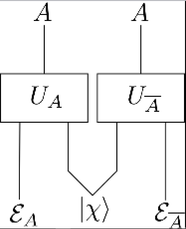
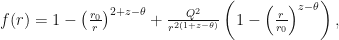
 , Kedar discusses his recent work, arguing that this further generalizes for hyperscaling violating Lifshitz theories (having a non-relativistic field theory dual).
 correspondence to non-relativistic holography. This involves working with hyperscaling voilating Lifshitz metric, which can be written as
![ds^2=\left(\frac{r}{r_{hv}}\right)^{-\theta}\left[-\frac{r^{2z}}{R^{2z}}dt^2+\frac{R^2}{r^2}dr^2 +\frac{r^2}{R^2}(dx^2+dy^2) \right],](https://s0.wp.com/latex.php?latex=ds%5E2%3D%5Cleft%28%5Cfrac%7Br%7D%7Br_%7Bhv%7D%7D%5Cright%29%5E%7B-%5Ctheta%7D%5Cleft%5B-%5Cfrac%7Br%5E%7B2z%7D%7D%7BR%5E%7B2z%7D%7Ddt%5E2%2B%5Cfrac%7BR%5E2%7D%7Br%5E2%7Ddr%5E2+%2B%5Cfrac%7Br%5E2%7D%7BR%5E2%7D%28dx%5E2%2Bdy%5E2%29+%5Cright%5D%2C&bg=ffffff&fg=111111&s=0&c=20201002)
 and
and  this reduces to the
  metric. The interest in such bulk theories stems from the fact that diffeomorphisms, which are the symmetry of this action, scale the time and the boundary coordinates
  differently. In general there can also be a horizon in the bulk,
![ds^2=\left(\frac{r}{r_{hv}}\right)^{-\theta}\left[-\frac{r^{2z}f(r)}{R^{2z}}dt^2+\frac{R^2}{r^2f(r)}dr^2 +\frac{r^2}{R^2}(dx^2+dy^2) \right],](https://s0.wp.com/latex.php?latex=ds%5E2%3D%5Cleft%28%5Cfrac%7Br%7D%7Br_%7Bhv%7D%7D%5Cright%29%5E%7B-%5Ctheta%7D%5Cleft%5B-%5Cfrac%7Br%5E%7B2z%7Df%28r%29%7D%7BR%5E%7B2z%7D%7Ddt%5E2%2B%5Cfrac%7BR%5E2%7D%7Br%5E2f%28r%29%7Ddr%5E2+%2B%5Cfrac%7Br%5E2%7D%7BR%5E2%7D%28dx%5E2%2Bdy%5E2%29+%5Cright%5D%2C&bg=ffffff&fg=111111&s=0&c=20201002)
 , thus introducing a temperature in the dual field theory. Of course, these do not seem to look like the solutions to vacuum Einstein’s equations and one needs to have quite an assortment of background
  gauge fields and matter fields which directly relate to the parameters
  in this metric. The action in four dimensions is,
![S=\int dx^4\sqrt{-g^{(4)}}\left[\frac{1}{16\pi G_4}\left(R-\frac{1}{2}\partial_M\Psi\partial^M\Psi+V(\Psi)-\frac{Z_1}{4}F_{1MN}F_1^{MN}\right)-\frac{Z_2}{4}F_{2MN}F_2^{MN}\right],](https://s0.wp.com/latex.php?latex=S%3D%5Cint+dx%5E4%5Csqrt%7B-g%5E%7B%284%29%7D%7D%5Cleft%5B%5Cfrac%7B1%7D%7B16%5Cpi+G_4%7D%5Cleft%28R-%5Cfrac%7B1%7D%7B2%7D%5Cpartial_M%5CPsi%5Cpartial%5EM%5CPsi%2BV%28%5CPsi%29-%5Cfrac%7BZ_1%7D%7B4%7DF_%7B1MN%7DF_1%5E%7BMN%7D%5Cright%29-%5Cfrac%7BZ_2%7D%7B4%7DF_%7B2MN%7DF_2%5E%7BMN%7D%5Cright%5D%2C&bg=ffffff&fg=111111&s=0&c=20201002)

 is chosen to get the asymptotic behaviour of the metric right, while
  imparts electric charge
  and
and  are related to
  in quite a cumbersome manner.
 , the
, the  .
.  being the transverse area of the brane.
 times something near the horizon. Doing a dimensional reduction yields,
 ,
,  take a particular value.
 and the matter field
  , one looks at the fluctuations,
 . These fluctuations satisfy the linearized equations of motion which come from the quadratic part of the action expanded about the background
  . Here
  is the on-shell value of the action for background solution and therefore the
  vanishes on-shell while
  determines the equations of motion for the above fluctuations.
![S[g_{\mu\nu}] = S_{EH} + \int_{bdy} d^{d-1}x \mathcal{L}(g_{\mu\nu}\partial g_{\mu\nu}).](https://s0.wp.com/latex.php?latex=S%5Bg_%7B%5Cmu%5Cnu%7D%5D+%3D+S_%7BEH%7D+%2B+%5Cint_%7Bbdy%7D+d%5E%7Bd-1%7Dx+%5Cmathcal%7BL%7D%28g_%7B%5Cmu%5Cnu%7D%5Cpartial+g_%7B%5Cmu%5Cnu%7D%29.&bg=ffffff&fg=111111&s=0&c=20201002)
 ), and a naive variation would produce contributions from the boundary of the manifold. These surface contributions would contain not just the variation of the metric
  , but also of its derivative
  . Then, setting
  becomes insufficient to kill all surface terms and the variation of the GHY term exactly cancels all terms involving
  enhances to a Virasoro
  Virasoro, which is an infinite dimensional asymptotic symmetry group. This statement creates many happy faces in the audience as they are finally able to see the missing link – Virasoro algebra in
  more visible than before.
 , which he proceeded to use to find Cardy’s formula which gives the density of asymptotic states,

 , where
  is the horizon of the BTZ black hole – you might remember this formula from his second lecture. He remarked that this paper was probably the most cited and important paper in theoretical high energy physics which doesn’t contain a single new equation!
 correspondence at the crossroads, fully awoken from the thrill of the lecture, we headed for lunch.
 is the reduced density matrix obtained by partial tracing over complement of
 is the surface with minimal area in the bulk and which ends on the boundary of
  expansion of the entanglement entropy was obtained. It carried the interpretation of measuring the amount of entanglement of the region enclosing the RT surface and the rest of the bulk.
 and
and  . He also noted that the HKLL prescription described to us by Nirmalaya was employed causal wedges and a prescription using entanglement wedges can be constructed, but turns out to be harder.
 implies that quantum fluctuations are supressed.
 to create a massive bulk field, whilst avoiding back-reaction in the bulk.
 .
. independent constants of motion, which also Poisson commute among themselves. He pointed out that one generally finds integrable systems for
  . A consequence, hence, is that most systems in nature (with a large number of degrees of freedom) tend to be chaotic, and one already begins to see inklings of why
  , where
  is the Lyaponov exponent. Via AdS/CFT, this translates to the statement that in a black hole background, gravitational perturbations exhibit maximal chaos.
![\frac{\delta q(t)}{\delta q(0)}={q(t),p}=\exp[\lambda T],](https://s0.wp.com/latex.php?latex=%5Cfrac%7B%5Cdelta+q%28t%29%7D%7B%5Cdelta+q%280%29%7D%3D%7Bq%28t%29%2Cp%7D%3D%5Cexp%5B%5Clambda+T%5D%2C&bg=ffffff&fg=111111&s=0&c=20201002)
![\frac{-i}{\bar{h}}[q(t),p]=\exp[\lambda T].](https://s0.wp.com/latex.php?latex=%5Cfrac%7B-i%7D%7B%5Cbar%7Bh%7D%7D%5Bq%28t%29%2Cp%5D%3D%5Cexp%5B%5Clambda+T%5D.&bg=ffffff&fg=111111&s=0&c=20201002)
![[W(t), V (0)]](https://s0.wp.com/latex.php?latex=%5BW%28t%29%2C+V+%280%29%5D&bg=ffffff&fg=111111&s=0&c=20201002) between a pair of Hermitian operators. This commutator represents the sensitivity of
between a pair of Hermitian operators. This commutator represents the sensitivity of  to perturbations created at an initial time by
  . The strength of this effect is measured by the thermal average,
![c(t)=-\langle[W(t),V(0)]^2\rangle_{\beta},](https://s0.wp.com/latex.php?latex=c%28t%29%3D-%5Clangle%5BW%28t%29%2CV%280%29%5D%5E2%5Crangle_%7B%5Cbeta%7D%2C&bg=ffffff&fg=111111&s=0&c=20201002)


 is the dissipation time. The chaotic behavior of
  can be probed by the out of time order correlator (OTOC),
 . Since, there were some questions regarding why this should vanish at large time dynamics, Avik proceeded to offer some plausibility arguments.
 (on the CFT side). Mathematically, within the time scale
  , the OTOC can be written as:
![\langle W(t)V W(t)V\rangle = 1-\frac{f_{0}}{N^{2}}\exp\bigg[\frac{2N}{\beta}t\bigg],](https://s0.wp.com/latex.php?latex=%5Clangle+W%28t%29V+W%28t%29V%5Crangle+%3D+1-%5Cfrac%7Bf_%7B0%7D%7D%7BN%5E%7B2%7D%7D%5Cexp%5Cbigg%5B%5Cfrac%7B2N%7D%7B%5Cbeta%7Dt%5Cbigg%5D%2C&bg=ffffff&fg=111111&s=0&c=20201002)
 is the inverse temperature and
  is a positive order one constant that depends on the specific operators V and W. The time at which the second term becomes relevant gives the scrambling time as,

![\bigg\langle e^{\int_{\partial AdS}\phi_0^i\mathcal{O}_i}\bigg\rangle \approx e^{-S_{AdS}[\phi_i]},](https://s0.wp.com/latex.php?latex=%5Cbigg%5Clangle+e%5E%7B%5Cint_%7B%5Cpartial+AdS%7D%5Cphi_0%5Ei%5Cmathcal%7BO%7D_i%7D%5Cbigg%5Crangle+%5Capprox+e%5E%7B-S_%7BAdS%7D%5B%5Cphi_i%5D%7D%2C+&bg=ffffff&fg=111111&s=0&c=20201002)
 s are dual CFT operators corresponding to the bulk fields
  . The non-normalisable mode of the bulk field evaluated at the boundary
  acts as the source for the CFT operator. To calculate the connected part of the CFT correlation functions, one has to take functional derivatives of the CFT partition function w.r.t. sources
  are regular at the black hole horizon, and there is a question of choice.
  that can be constructed by taking the quotient of the complex plane
  with a lattice. Orbifolded spacetimes can have conical singularities in them that are naked singularities. These can be interpreted as alluding to the presence of some massive particle in
  of the two torii corresponding to the thermal
  . This relation between the two torii geometries will be explicitly used to derive the
  , the BTZ black hole partition function dominates over the thermal
  , it is the thermal AdS’ turn to dominate over BTZ. At
  , there is a first order phase transition due to a jump in the first derivative of the free energy. This can be visualised as an interchanging of cycles of the two torii. This phase transition is famously known as the
  may be expressed as,
 is the “smearing function.”

 . For the interacting field theory we considered above, one may now obtain the final form of the field
 is an embedded submanifold of
  with the metric,
 and
and  parametrize a subregion of the full
  in this wedge. The field
 and
and  are the AdS-Rindler wedge and its intersection with the AdS boundary respectively. It is important to note that
  which transforms under the conformal generators as a bulk field. It was shown that the isometries
  and
and  keep the origin fixed in the bulk as
  and
and  . Next, an ansatz was made to express the above bulk field in terms of all the descendant fields of the primaries in the CFT as,
 . So, in this way, one may obtain the desired bulk scalar field from Nakayama-Ooguri method.
 i.e., the standard deviation of the couplings, followed by the introduction of a delta function which was then smeared. This is somewhat akin to the Fadeev-Popov method of quantization in the context of non-Abelian gauge theories. In the course of this evaluation, he introduced the two point correlator and eventually got to the Schwinger-Dyson equations,
 is the contribution from self-energy processes while
  and
and  are the Green’s function of the free theory and the full interacting theory respectively. The most natural step after this was to connect it with the popular diagramatic representations known as ‘melonic diagrams’ (frankly, these look more like pumpkins than melons). A crucial point he highlighted was the fact that these melonic diagrams contribute because of the large
  , where

 or
or  for these lectures. The equation above is a claim regarding the equality of certain gravitational theories to certain field theories. (AdS stands for Anti de Sitter spacetime, and CFT for Conformal Field Theory). Even though originally this was discovered (conjecturally) by Maldacena as an equality between maximally supersymmetric Yang-Mills theory in four dimensions and type IIB string theory on
  , we were told we will concentrate on
  . Why
. Why  for
for  ) and the Ricci tensor (
 ) have the same number of independent components. In particular, we saw that the Riemann tensor, which captures the information about the geometry, can be written in terms of the Ricci tensor, which is determined (in the case of two-derivative theories) by Einstein’s equations to be proportional to the metric.
 in higher dimensions, two dimensional CFTs enjoy infinite number of symmetry generators. We can use complex analysis for the two dimensional theory, we can use ‘modular invariance’, there exists minimal models where even without knowing the Lagrangian, one can write the correlators!
 gauge theories. t’Hooft’s double line notation was introduced briefly and we saw by examples that if we do a
  as the parameter of the theory, only planar diagrams appear in the leading order. Several members of the audience went upto the board before everyone was convinced that if the double line diagram rules are followed, non planar diagrams can not be written as planar diagrams.
 . i.e. one can make a saddle point approximation at large
  and
and  . This mapping of couplings would set the stage for the holographic dictionary to be used in the future lectures.
 -dimensions is dual to CFT in $d$-dimensions that lives on the boundary of AdS (also referred to as bulk). Also, the map between various quantities on both sides is given by AdS/CFT dictionary. According to this dictionary, any bulk geometry (
 ) is mapped to a specific state in CFT (
 ). (One simple example is that the pure AdS maps to the vacuum of the CFT.) Further, the correlators in the bulk are mapped to that of the boundary as follows:
 and
and  are bulk and boundary coordinates respectively and
  is the scaling dimension of the operator
  .
.  , we are reaching the boundary. Also,
 is a scalar field in AdS of mass
  . It satisfies the Klein-Gordon equation in AdS i.e.,
  . This equation admits the solution of the following form:
 are the two independent plane wave solutions of the Klein-Gordon equation. Now, following the extrapolate dictionary, we impose the boundary condition:
  . Using the orthogonality of
 with a similar expression for
  . $g_{n,l,m}$ is defined by the following relation:
  . Writing
  for shear diffusion (where
  is the shear diffusion constant) arises as a pole in the correlation function of stress tensor components
  and the shear viscosity is computed by the Kubo’s formula
![\eta=-\lim_{\omega\rightarrow 0} \frac{1}{\omega}\int d^d x e^{i\omega t} \theta(t)\langle[T_{xy}(x),T_{xy}(0)]\rangle\](https://s0.wp.com/latex.php?latex=%5Ceta%3D-%5Clim_%7B%5Comega%5Crightarrow+0%7D+%5Cfrac%7B1%7D%7B%5Comega%7D%5Cint+d%5Ed+x+e%5E%7Bi%5Comega+t%7D+%5Ctheta%28t%29%5Clangle%5BT_%7Bxy%7D%28x%29%2CT_%7Bxy%7D%280%29%5D%5Crangle%5C+&bg=ffffff&fg=111111&s=0&c=20201002)
 as a perturbation on
  background. Solving the scalar field equation
  of dimension
  couples to
  . Then using the linear response theory described above, we compute the
  . Also computing the entropy density for the black brane in
  (in relativistic units), which saturates the viscosity bound proposed by Kovtun, Son and Starinets


 .
. are required to be Cartan-valued, and further that the gauge field
  and auxiliary scalar
